Taeyang Yang님의 블로그 와 StatQuest의 유튜브 를 참조하였다.
AdaBoost
AdaBoost(Adaptive Boosting)는 다양한 크기의 Stump로 이루어진 숲이다.
3 Concepts of AdaBoost
- Forest of stumps : weak learner로 구성된 숲
- Different weights for each stump : Amount of Say의 양
- Sequential : 각 stump의 에러가 다음 stump의 에러에 영향을 미친다.
1. Forest of stumps
random forest에서는 개별 모델로 decision tree를 사용하는데 비해,AdaBoost에서는 개별 모델로 Stump
를 사용한다. Stump란 한 노드와 두 개의 가지를 갖는 decision tree 로 정의할 수 있다.

여러 질문을 통해 데이터를 분류하는 의사결정나무와 다르게 stump는 정확한 분류를 하지 못한다. stump는 하나의 질문으로 데이터를 분류해야 하기 때문. 따라서 stump는 weak learner라고 할 수 있다.
2. Different weight for each stump


random forest에서 모든 tree는 동일한 weight를 통해 결과를 산출한다.
반면, AdaBoost에서 각 stump는 서로 다른 weight(amount of say)를 갖는다. 즉, 최종 앙상블 시 개별 모델마다 예측 결과값에 가중치를 달리 부여한다.
3. Sequential

Random forest에서 tree 들은 parallel하게 만들어진다. 즉, decision tree간 서로 영향이 없다.
반면, AdaBoost에서 stump들은 sequential하게 만들어진다는 특징을 갖는다. 즉, 기존에 만들어진 stump가 이후 만들어질 stump에 영향을 준다.
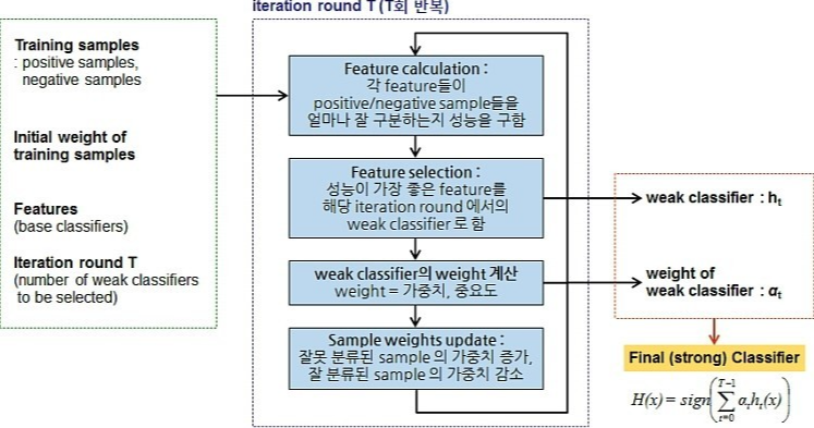
AdaBoost 학습 순서
1. Initial sample weight

initial sample weight는 모두 동일하게 해준다.
$$Initial sample weight = w_{i, 1} = {1\over total number of samples}$$
* $\Sigma Initial sample weight = 1$
2. First stump

Impurity(Gini index)를 바탕으로 best arrtibute로 분기하는 stump를 찾는다.
3. Amount of say

완성한 stump의 분류 결과에 따라 amount of say $\alpha_t$를 계산해준다. $\alpha_t$는 각 앙상블 시 각 모델의 예측값 $h_t$에 대한 가중치로 사용된다.$$말의 양 = \alpha_t = {1\over2}log({1-\epsilon_t}\over \epsilon_t)$$
- $\epsilon_t$ : Total error로, 오분류된 샘플의 sample weight 총합으로 정의
$$\epsilon_t = \Sigma_{i=1}^n w_{i, t} , h_t(x_i) \neq y_i$$
전체 sample weights의 총 합이 1이기 떄문에 최고의 stump를 만들 경우(모두 맞춤) $\epsilon_t = 0$, 반대로 최악의 stump를 만든 경우(모두 틀림) $\epsilon_t = 1$을 갖는다.

또한, $\epsilon_t$에 따른 $\alpha_t$의 변화를 그림으로 그려보면, $\epsilon_t$가 낮을 때(<0.5)는 양의 $\alpha_t$를, $\epsilon_t$가 높을 때는 (>0.5) 음의 $\alpha_t$를 갖는다. 또한 $|\alpha_t|$는 $\epsilon_t$가 극단적인 값일수록(0 or 1에 가까울수록) 더욱 커진다.
위 예시의 amount of say $\alpha_t= 0.97$
4. Updated sample weight
각 sample weight $w_{i, t}$를 $w_{i, t+1}$로 업데이트한다.여기서 핵심은 오분류된 sample의 weight는 늘리고, 정분류된 sample의 weight는 낮춰주어야 한다.
4.1. 오분류된 샘플
$$New sample weight = w_{i, t+1} = w_{i, t} \times e^{\alpha_t}$$
4.2. 정분류된 샘플
$$New sample weight = w_{i, t+1} = w_{i, t} \times e^{-\alpha_t}$$
4.3. 정규화 (총합 = 1)
$$Normalized smaple weight = {New sample weight \over \Sigma New sample weight}$$
따라서 새로운 $w_{i, t+1}$을 얻는다. 오분류된 샘플은 가중치가 (${1\over8} = 0.125$에 비해 높아진 반면, 나머지 샘플들은 가중치가 낮아진 것을 확인할 수 있다.

5. Next stump
업데이트된 sample weight를 적용한 새로운 stump를 만든다. 분기 시 impurity를 계산할 때 두가지 방법으로 sample weight를 적용할 수 있다.
5.1. Weighted Gini index
sample weight를 각 sample에 적용하여 gini index를 계산한다.
$$Weighted Gini index = \Sigma_{i=1}^C w_{i, t} \times p_i(1-p_i)$$
5.2. Resampling
중복을 허용하여 dataset을 resampling 후 gini index를 계산한다.

- sample weight를 바탕으로 0~1의 구간을 나눈다.
- 0~1 값을 원래 샘플 수 만큼 random sampling하고, 이 값에 따라 원 데이터에서 데이터를 다시 sampling
- sample weight가 큰 경우, 더 넓은 구간을 가지고 -> 해당 샘플이 더 자주 뽑힌다.
위 그림처럼 오분류된 샘플이 많이 포함된 새로운 데이터셋이 만들어지고, sample weight는 다시 ${1 \over total number of samples}$로 초기화 된다. * sample weight는 같아도, 동일한 샘플이 더 많이 있기에, 결과적으로 sample weight가 다른것과 동일한 효과
6. Repetition

정해진 iteration만큼 stump가 생성될 때까지 3~5 과정을 반복
7. 최종 예측

$N$번의 iteration을 진행 후, 모든 stump의 예측값 $h_t(x)$에 amount of say $\alpha_t$를 가중치로 곱하는 hard voting을 통해 최종 예측값을 얻어낸다.
$$F(x) = \Sigma_{t=1}^N \alpha_t h_t(x)$$
요약

참조
- Viola, P., & Jones, M. J. (2004). Robust real-time face detection. International journal of computer vision, 57(2), 137-154.
- https://bkshin.tistory.com/entry/%EB%A8%B8%EC%8B%A0%EB%9F%AC%EB%8B%9D-14-AdaBoost
- https://tyami.github.io/machine%20learning/ensemble-3-boosting-AdaBoost/
- https://www.youtube.com/watch?v=LsK-xG1cLYA
'Machine Learning' 카테고리의 다른 글
| 클러스터링 평가 지표(Clustering Evaluation Metrics) (0) | 2022.09.19 |
|---|---|
| 배깅 앙상블 (Bagging Ensemble): Random Forest (0) | 2022.04.04 |
| 앙상블 (Ensemble)의 개념 (1) | 2022.04.04 |
| 의사결정 나무 (Decision Tree) ID3 알고리즘 (0) | 2022.04.04 |
| 의사결정나무, Decision Tree (0) | 2022.04.04 |


댓글